Implemented Kernel Functions
-
2D Cubic Spline Kernel for \(\kappa = 2h,\, \alpha = \frac{5}{14 \pi h^2}, \, r=\lVert\mathbf{\vec{x}}_{ij}\rVert, \, q=\frac{r}{h}\) :
\[W_{\text{spline}}(\mathbf{\vec{x}}_{ij}) := \alpha \begin{cases} (2-q)^3 - 4(1-q)^3& 0 \leq q < 1\\ (2-q)^3 & 1 \leq q < 2\\ 0 & q \ge 2 \end{cases}\] \[\nabla W_{\text{spline}}(\mathbf{\vec{x}}_{ij}) := \alpha \frac{\mathbf{\vec{x}}_{ij}}{\lVert\mathbf{\vec{x}}_{ij}\rVert h}\begin{cases} -3(2-q)^2 +12 (1-q)^2& 0 \leq q < 1\\ -3(2-q)^2 & 1 \leq q < 2\\ 0 & q \ge 2 \end{cases}\]- Vanishing gradients as \(r\to 0\) problematic for pressure computation?
-
2D Spiky Kernel suggested by Müller, Charypar, Gross after Desbrun, Cani normalized for 2D for \(\kappa = 2h,\, \alpha = -\frac{10}{\pi\kappa^5}, \, r=\lVert\mathbf{\vec{x}}_{ij}\rVert\) :
\[W_{\text{spiky}}(\mathbf{\vec{x}}_{ij}) := \alpha \frac{\mathbf{\vec{x}}_{ij}}{\lVert\mathbf{\vec{x}}_{ij}\rVert}\begin{cases} (\kappa-r)^3& 0 \leq r \leq \kappa\\ 0 & \text{otherwise} \end{cases}\] \[\nabla W_{\text{spiky}}(\mathbf{\vec{x}}_{ij}) := \alpha \frac{\mathbf{\vec{x}}_{ij}}{\lVert\mathbf{\vec{x}}_{ij}\rVert}\begin{cases} (\kappa-r)^2& 0 < r \leq \kappa\\ 0 & \text{otherwise} \end{cases}\]- Unrealistic viscous behaviour?
- Wrong density estimation for ideal sampling?
-
2D Double Cosine Kernel proposed by [Yang, Peng,Liu] for \(\kappa = 2h,\, \alpha = \frac{\pi}{(3\pi^2-16)(\kappa)^2}, \, r=\lVert\mathbf{\vec{x}}_{ij}\rVert, \, s=\frac{r}{h}\):
\[W_{\text{cos}}(\mathbf{\vec{x}}_{ij}) := \alpha \begin{cases} 4\cos(\frac{\pi}{2}s)+\cos(\pi s)+3& 0 \leq s \leq 2\\ 0 & \text{otherwise} \end{cases}\] \[\nabla W_{\text{cos}}(\mathbf{\vec{x}}_{ij}) := \alpha \frac{\mathbf{\vec{x}}_{ij}}{\lVert\mathbf{\vec{x}}_{ij}\rVert}\begin{cases} -2\frac{\tau}{\kappa}\sin(\frac{\pi}{2}s)-\frac{\tau}{\kappa}\sin(\pi s)& 0 \leq s \leq 2\\ 0 & \text{otherwise} \end{cases}\]
Kernel Function Plots
Kernel Functions for \(\kappa = 2h,\, h=1\)
- Surprisingly equal integral? Projection to 1D may be at fault, outer regions weigh quadratically more in 2D integral
Magnitude of Kernel Gradient over \(\mathbf{\vec{x}}_{ij}\) for Cubic Spline and Spiky Kernel:
Testing the Kernel Function
- Kernel properties are tested
- Integrals are implemented with Monte Carlo, \(N=10^{8}\) on \(\Omega=[-2.1h; 2.1h]\)
- Accepted error is \(\epsilon = 10^{-3}\)
- They are checked again with Riemann sums of \(n=10^4,\, \epsilon=10^{-9}\)
- All other tests are run \(N\) times with random \(\mathbf{\vec{x_i}, \vec{x_j}}\)
-
For ideal sampling, where \(\kappa = 2h\), \(h\) is the particle spacing a regular grid is used for \(\mathbf{\vec{x}}_j\):
\[\begin{align} \sum_j&W(\lVert \mathbf{\vec{0} - \vec{x_j}} \rVert, \kappa) = \frac{1}{h^2}&&\text{Integral is Density}\\ \sum_j&\nabla W(\mathbf{\vec{0} - \vec{x_j}}, \kappa) = \mathbf{\vec{0}}&&\text{Gradient Integral is Zero}\\ \sum_j &\left(\mathbf{(\vec{0} - \vec{x}_j)} \odot \nabla W_{ij} \right) = -\frac{1}{V} \cdot \mathbf{\vec{1}}&&\text{Gradient Normalization} \end{align}\] - On a \(100\times 100\) regular grid and a random grid, the consistency of each \(\nabla W\) is tested by comparing to a \(\mathcal{O}(\Delta x^4)\) central difference of \(W\) with an accepted error of \(1\%\)
- ❌ this fails for Cubic Spline for small \(h\) - numerical problem at discontinuity?
- ❌ always fails for Spiky kernel - smoothness too low?
- ✅ always passes for Double Cosine kernel
Failed Tests
❌ Ideal Sampling: \(\sum_j \left(\mathbf{(\vec{x}_i - \vec{x}_j)} \odot \nabla W_{ij} \right) = -\frac{1}{V} \cdot \mathbf{\vec{1}}\) always fails
| Kernel | Failed Tests |
|---|---|
| Cubic Spline ❓ | \(W\) and \(\nabla W\): consistency with finite difference? |
| Spiky Kernel ❌ | Ideal Sampling: \(\int_{\mathbf{x_j}\in[-\kappa;\kappa]^2}W(\lVert \mathbf{\vec{0} - \vec{x_j}} \rVert, \kappa) = \frac{1}{h^2}\) off by +27.36% |
| Double Cosine ✅ | None |
Stability as an interval over stiffness \(k\)
- Viscosity: Double Cosine Kernel
- Pressure and Density Computations: Cubic Spline or Double Cosine
- Instability for \(\nu=0.02, h=0.03, \lambda=0.1\) is defined as:
- when a watter column of height \(3\) in a \(3\times 3\) box has \(\epsilon_{\rho}>5\%\) density deviation
- or starts oscillating at the bottom boundary
- Results:
- Double Cosine stable for \(k\in[580; 2400]\)
- Cubic Spline stable for \(k\in[18200; 93000]\)
Double Cosine Kernel for \(k=580\) and \(k=2000\) (unstable on the left, stable on the right)
Testing Energy Conservation
The Hamiltonian is for now defined as :
\[\mathcal{H} = \sum_i^N \left( m_i \mathbf{\vec{g}} \cdot \mathbf{\vec{x}}_i + \frac{1}{2} m_i \mathbf{\vec{v}}_i \cdot \mathbf{\vec{v}}_i\right)\]And normalized as \(\mathcal{H}_{min} = mgh_{min}\) and \(\mathcal{H}_{norm} = \frac{\mathcal{H}-\mathcal{H}_{min} }{\lVert \mathcal{H}_{min} \rVert}\) for plotting
but appears to be missing a term that is proportional to the compression of the fluid (internal energy potential?) as indicated by oscillations in a resting water column:
- Should \(U =\sum_i^N p_i V_i = p_i\frac{m_i}{\rho_i}\) be used to compensate? Can the oscillation even be avoided?
Improving the Acceleration Datatructure
+400 FPS@N=4k / +60%
- Filter by \(\lVert \mathbf{\vec{x_i} - \vec{x_j}} \rVert \le \kappa\) when building neighbour lists instead of saving supersets with all particles in neighbouring grid cells. ~15%@N=4k
- Binary search directly in particle handles, don’t build a compact list of filled cells like suggested in Compressed Neighbor Lists for SPH (???). ~30%@N=4k
- Use an XYZ curve that is faster to compute than a Morton Code (?) ~15%@N=4k
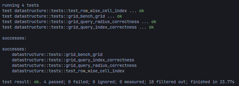
Testing the Acceleration Datatructure
For \(\kappa \in [0.9, 1.0, 1.1], \, N=5000\) particles are randomly distributed in \([-10;10]\) and the neighbour sets for each compared to the ones computed per brute force in \(\mathcal{O}(n^2)\). This is repeated 10 times. ✅
Current State of the Project
Questions
- What does \(\sum_j \left(\mathbf{(\vec{x}_i - \vec{x}_j)} \odot \nabla W_{ij} \right) = -\frac{1}{V} \cdot \mathbf{\vec{1}}\) actually mean? Why does it always fail for ideal sampling?
- Why did the test for the spiky kernel fail?
- Why do the stable parameters differ so wildly from kernel to kernel?
- Why did not producing a compact filled cell list improve neighbour search performance? (size of the system?)
- How can energy conservation accurately be tracked?
Conclusions - After the Meeting
- \(\sum_j \left(\mathbf{(\vec{x}_i - \vec{x}_j)} \odot \nabla W_{ij} \right) = -\frac{1}{V} \cdot \mathbf{\vec{1}}\) actually worked! Error tolerances were to low
- Cubic Spline has 1.3% error, as expected
- Double Cosine has 4.7% error
- The gradients are now normalized such that this error is zero by applying a constant factor.
-
Remove consistency check with finite difference
-
The Spiky Kernel was removed from the simulation.
- Kernel normalization in the Cubic Spline kernel was off by a factor of \(\frac{1}{h}\) because of an error in the slides that was copied (p.64).
- this was neatly demonstrated in the “Stability as an interval over stiffness k”-Section, where the interval for k was off by exactly \(\frac{1}{h}=\frac{1}{0.03}=33\frac{1}{3}\)