Towards a single non-uniform layer
Single uniform layer
- Following the 2019 SPH Tutorial, we define for a particle ideally surrounded by fluid on a single layer of boundary particles:
- \[\begin{align} \gamma_1 &:= \frac{V_i - \sum_{i_f}W_{i,i_f}}{\sum_{i_b} W_{i, i_b}} = \frac{\frac{1}{h^2} - \sum_{i_f}W_{i,i_f}}{\sum_{i_b} W_{i, i_b}}\\ \\ \gamma_2 &:= \frac{\sum_{i_f}\nabla W_{i,i_f} \cdot \sum_{i_b} W_{i, i_b}}{\sum_{i_b} W_{i, i_b} \cdot \sum_{i_b} W_{i, i_b}} \end{align}\]
- This turns out to be \(\gamma_1, \gamma_2 = 1\) for a Cubic Spline with \(h=2\) in 2D
- Higher \(\gamma_2\) decreases stability, the opposite seems true as well
- Higher \(\gamma_1\) seems to not decrease stability but improve impenetrability
Single non-uniform layer
Scrapping the use of \(\gamma_1\) in the density computation and instead calculating \(m_{i_b}\) works as described:
- \[\rho_i = m_i\sum_{i_f} W_{i,i_f} + \sum_{i_f} m_{i_b}W_{i,i_b}\]
- \[m_{i_b} = \rho_0 \cdot V_{0, i_b} =\rho_0 \frac{\gamma_1}{\sum_{i_{b_b}}W_{i_b, i_{b_b}}}\]
- Add image-based initialization:
- blue pixels correspond to fluid
- black pixels are boundaries
- IT WORKS! ✅
\(\lambda = 0.01, k=1250, \nu=0.015\) with maximum compression \(\le 0.24\%\)
- Water levels equal out as they should:
\(\lambda = 0.1, k=1250, \nu=0.015\) with maximum compression \(\le 0.4\%\)
Jittered Initialization
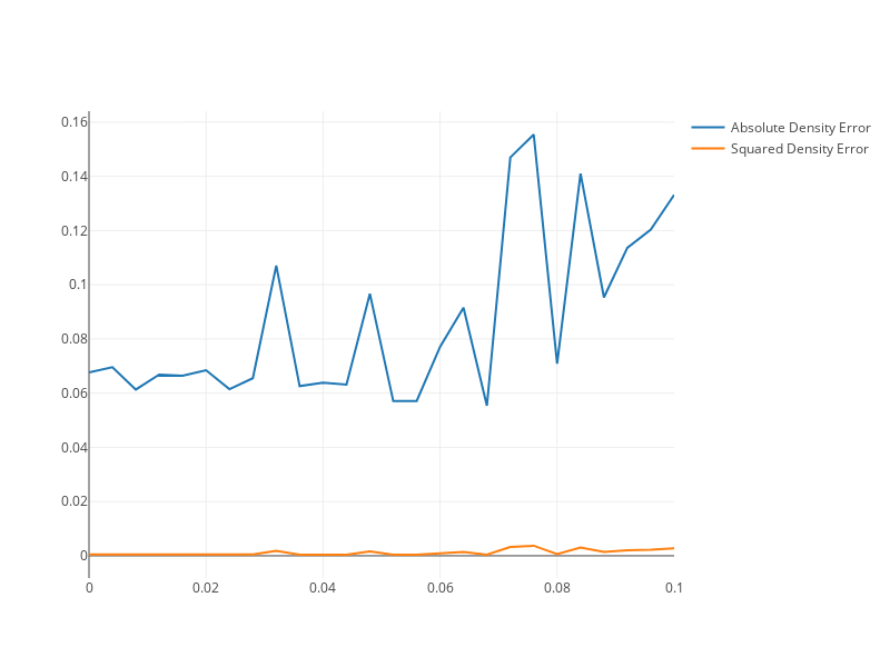
Introducing even just \(0.01h\) as random jitter when initializing particles can improve stability at the beginning of the simulation:
(example for \(h=0.05, k=2300, \nu=0.03\) water column height of \(1\), left is unjittered)
- not very predictable for low sampling resolutions
- the absolute and the squared density error \(E_{abs}, E_{sqrd}\) of a simulation are defined as:
- plotted against amount of initial random jitter in units of the particle spacing \(h\) for \(h=0.05, k=2000, \nu=0.03\):
- in larger systems, small (\(0.01h\)) jitter effectively prevents aliasing artefacts:
(video slowed down x8 with motion interpolation, left is jittered \(N=90000, h=0.01, \lambda = 0.1, k=2000, \nu=0.01\))
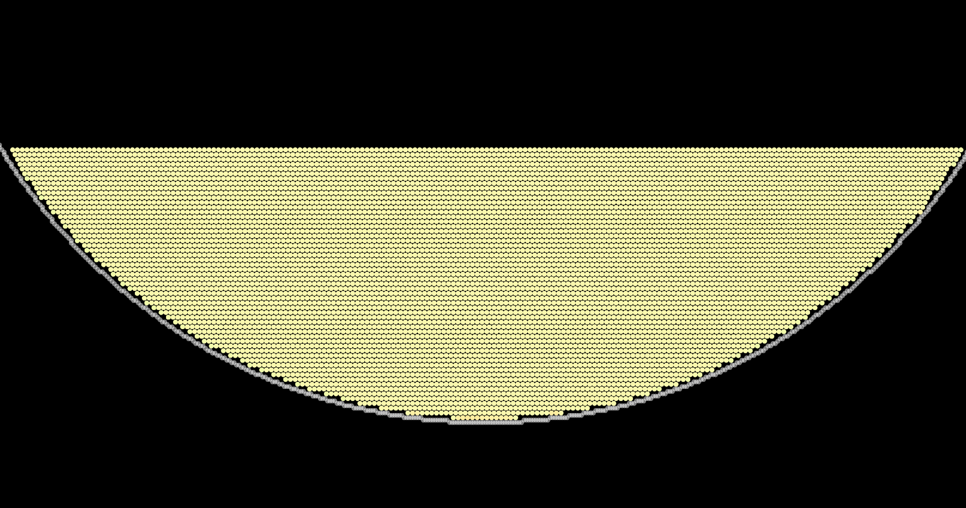
Mass Initialization
- density at \(t=0\):
- is highly inflated at ‘oversampled’ boundary
- is underestimated at the free surface
- produces a shockwave that leads to splashes
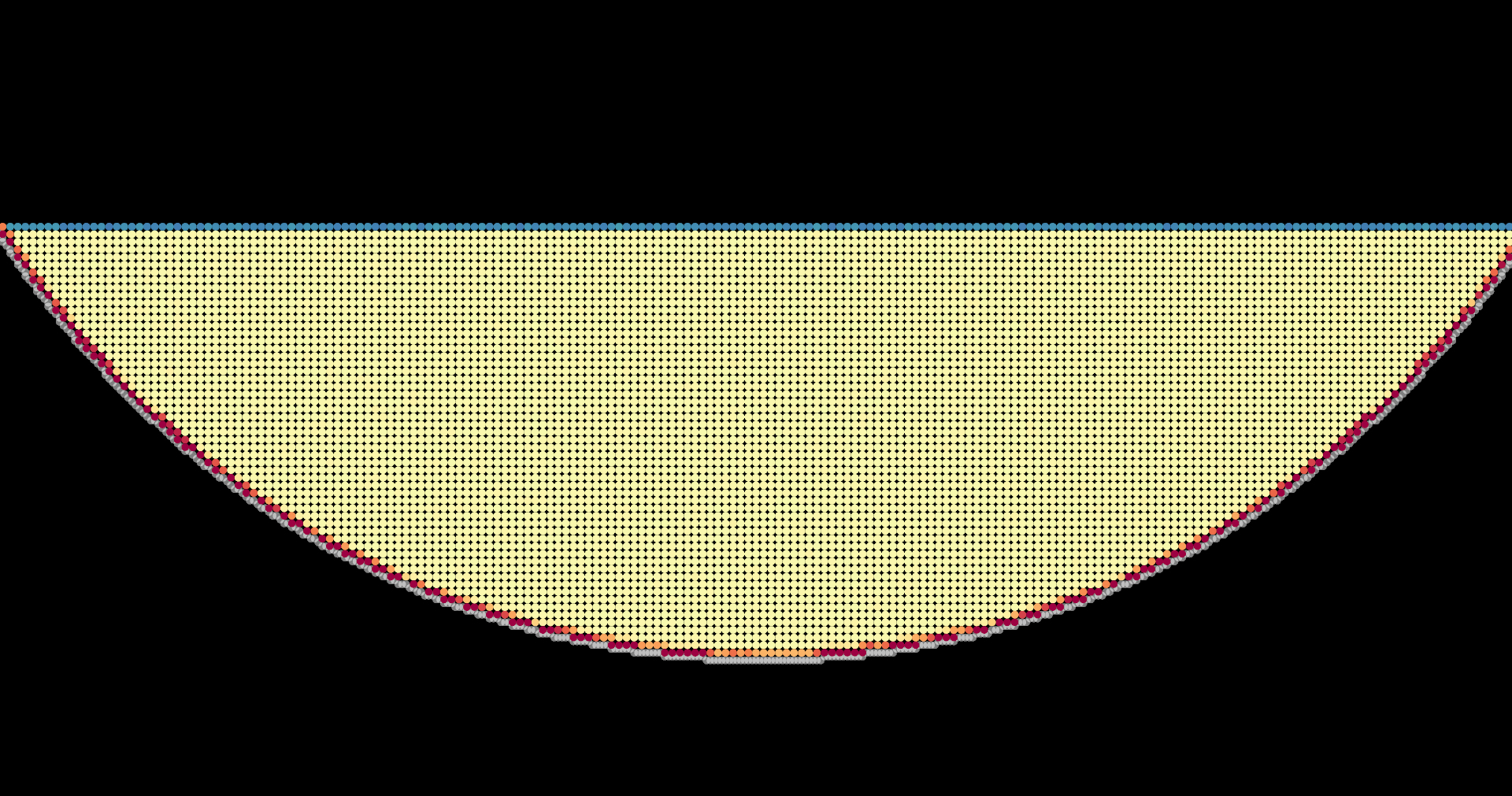
Countermeasures:
- initialize in hexagonal grid for more stability
- instead of \(m_i := h^2\) for \(\rho_0 = 1\), use:
- \[m_i = \frac{\rho_0}{\frac{1}{V_i}} = \frac{\rho_0}{\sum_{j_f}W_{ij_f} + \sum_{j_b}W_{ij_b} * \frac{m_{j_b}}{m_0}}\]
- don’t place fluid samples within \(h\) radius of a boundary sample
Problems
Weird type of instability for large \(k\)
- only for high values of \(k>1500\)
- especially for very low viscosities \(\nu \le 0.01\)
- only when water starts resting (here: \(t\ge 8.6s\))